- CodeCraft by Dr. Christine Lee
- Posts
- 12 Essential Data Analytics Functions for Beginners (Part 1)
12 Essential Data Analytics Functions for Beginners (Part 1)
Getting Started with Pandas

Data Analytics and Visualisation
Welcome back, Python enthusiasts! Today, we’re diving into the world of Pandas, one of the most powerful libraries for data manipulation and analysis. This post will introduce you to 12 essential Pandas functions that every beginner should know. We’ll explain key terminologies and provide real-life examples to make your learning experience fun and practical. Let’s get started!
What You Will Learn
Pandas Library: Introduction and its importance in data analysis.
Key Functions: Detailed explanation of 12 essential Pandas functions.
Real-Life Examples: Practical examples to illustrate each function.
Key Terminologies: Simple explanations of important terms.
Introduction to Pandas
Pandas is a Python library used for data manipulation and analysis. It provides data structures and functions needed to work on structured data seamlessly. The two primary data structures in Pandas are:
Series: A one-dimensional labeled array capable of holding any data type.
DataFrame: A two-dimensional labeled data structure with columns of potentially different types.
Key Terminologies
DataFrame: A table-like data structure with rows and columns.
Series: A single column of data, like a column in a spreadsheet.
Index: The labels of the rows in a DataFrame or Series.
CSV: Comma-Separated Values, a common file format for storing tabular data.
1. Reading Data with read_csv()
The read_csv() function is used to read a CSV file and convert it into a DataFrame.
Example:
import pandas as pd
# Reading data from a CSV file
df = pd.read_csv('sales_data.csv')
print(df.head())
Explanation:
pd.read_csv('sales_data.csv'): Reads the CSV file into a DataFrame.df.head(): Displays the first five rows of the DataFrame.
A sample data for sales_data.csv can be viewed from here.
2. Viewing Data with head() and tail()
The head() function displays the first few rows of a DataFrame, while the tail() function displays the last few rows.
Example:
# Displaying the first 5 rows
print(df.head())
# Displaying the last 5 rows
print(df.tail())
Explanation:
df.head(): Shows the first 5 rows of the DataFrame.df.tail(): Shows the last 5 rows of the DataFrame.
Output:

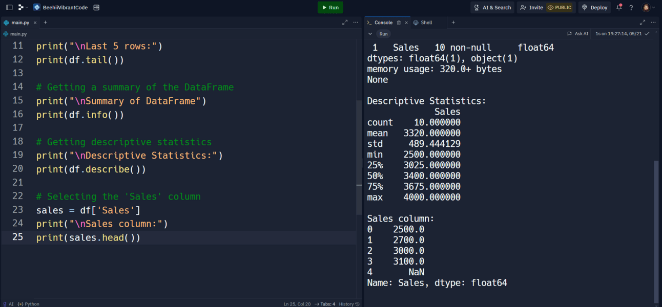
3. Getting Basic Information with info()
The info() function provides a concise summary of a DataFrame, including the number of entries, column names, data types, and memory usage.
Example:
# Getting a summary of the DataFrame
print(df.info())
Explanation:
df.info(): Displays a summary of the DataFrame.
Output:

4. Descriptive Statistics with describe()
The describe() function generates descriptive statistics for numerical columns, such as count, mean, standard deviation, min, and max values.
Example:
# Getting descriptive statistics
print(df.describe())
Explanation:
df.describe(): Provides descriptive statistics for numerical columns in the DataFrame.
Output:

5. Selecting Columns with []
You can select specific columns of a DataFrame using square brackets.
Example:
# Selecting the 'Sales' column
sales = df['Sales']
print(sales.head())
Explanation:
df['Sales']: Selects the 'Sales' column from the DataFrame.
Output:

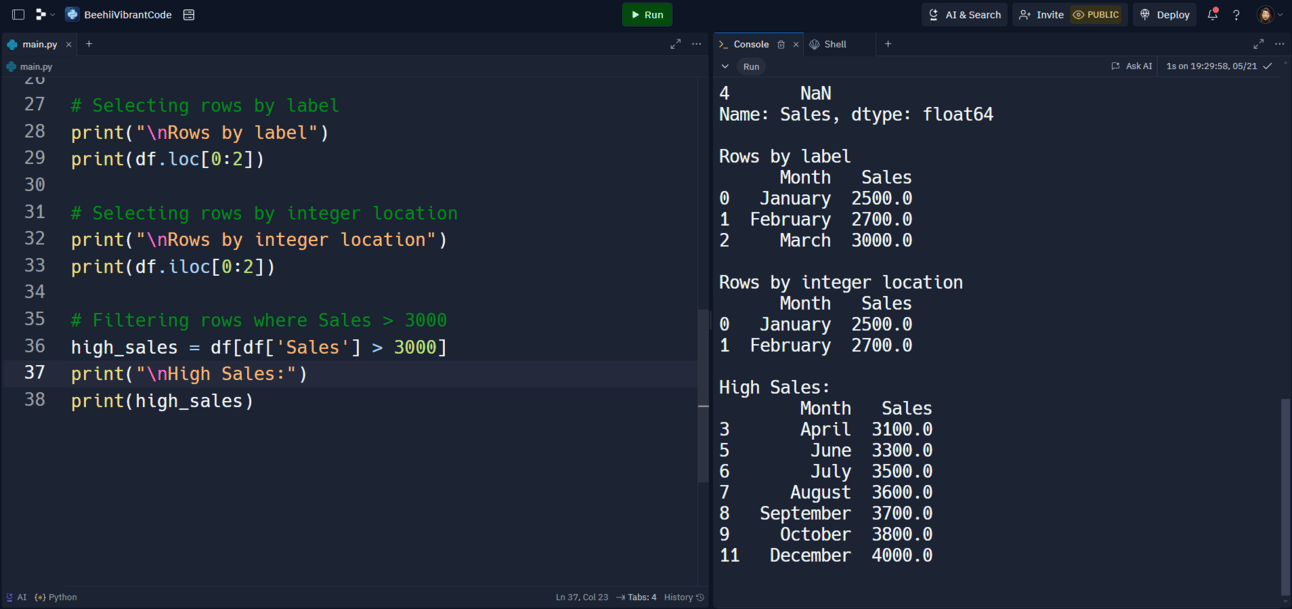
6. Selecting Rows with loc[] and iloc[]
The loc[] function selects rows based on labels, while the iloc[] function selects rows based on integer location.
Example:
# Selecting rows by label
print(df.loc[0:2])
# Selecting rows by integer location
print(df.iloc[0:2])
Explanation:
df.loc[0:2]: Selects rows 0 to 2 (inclusive) based on labels.df.iloc[0:2]: Selects rows 0 to 2 (exclusive) based on integer location.
Output:

7. Filtering Data with Conditions
You can filter data by applying conditions to DataFrame columns.
Example:
# Filtering rows where Sales > 3000
high_sales = df[df['Sales'] > 3000]
print(high_sales)
Explanation:
df[df['Sales'] > 3000]: Filters rows where the 'Sales' column values are greater than 3000.
Output:

8. Adding New Columns
You can add new columns to a DataFrame by assigning values to a new column name.
Example:
# Adding a new column 'Discounted_Price'
df['Discounted_Price'] = df['Sales'] * 0.9
print(df.head())
Explanation:
df['Discounted_Price'] = df['Sales'] * 0.9: Adds a new column 'Discounted_Price' with values 10% less than the 'Sales' column.
Output:

9. Removing Columns with drop()
The drop() function removes specified columns from a DataFrame.
Example:
# Removing the 'Discounted_Price' column
df.drop('Discounted_Price', axis=1, inplace=True)
print(df.head())
Explanation:
df.drop('Discounted_Price', axis=1, inplace=True): Removes the 'Discounted_Price' column from the DataFrame.
Output:

10. Sorting Data with sort_values()
The sort_values() function sorts the DataFrame by the values of a specified column.
Example:
# Sorting the DataFrame by 'Sales' in descending order
df_sorted = df.sort_values(by='Sales', ascending=False)
print(df_sorted.head())
Explanation:
df.sort_values(by='Sales', ascending=False): Sorts the DataFrame by the 'Sales' column in descending order.
Output:

11. Handling Missing Data with fillna()
The fillna() function fills missing values in a DataFrame with a specified value.
Example:
# Filling missing values in 'Sales' with the mean
df['Sales'].fillna(df['Sales'].mean(), inplace=True)
print(df.head())
Explanation:
df['Sales'].fillna(df['Sales'].mean(), inplace=True): Fills missing values in the 'Sales' column with the mean of the column.
Output:

12. Grouping Data with groupby()
The groupby() function groups the DataFrame using a column or columns and performs an aggregate function on each group.
Example:
# Grouping by 'Month' and calculating total sales
monthly_sales = df.groupby('Month')['Sales'].sum()
print(monthly_sales)
Explanation:
df.groupby('Month')['Sales'].sum(): Groups the DataFrame by the 'Month' column and calculates the sum of 'Sales' for each month.
Output:

Conclusion
Congratulations! You’ve just learned 12 essential Pandas functions that will help you manipulate and analyze data effectively. By understanding these functions and practicing with real-life examples, you’ll become proficient in using Pandas for data analysis.
Ready for More Python Fun
Subscribe to our newsletter now and get a free Python cheat sheet! Dive deeper into Python programming with more exciting projects and tutorials designed just for beginners.
Keep exploring, keep coding, and enjoy your journey into data analytics with Pandas!