7 Popular Pandas Functions for Data Analysis

Welcome back to our Pandas series! Today, we're going to explore some of the most commonly used Pandas functions for data analysis. These functions will help you load, clean, analyze, and visualize your data efficiently. Each function is accompanied by real-life examples and detailed explanations to make your learning experience practical and straightforward. Let’s get started!

 Recommendation and Inspiration

Sample dataset

Below is a sample dataset for sales_data.csv that you can use for the examples provided in the article. This dataset includes columns for TransactionID, Date, Store, Product, Quantity, and Price.

Sample Data for sales_data.csv

TransactionID,Date,Store,Product,Quantity,Price

1,2023-01-01,Store A,Laptop,1,1000

2,2023-01-01,Store A,Tablet,2,500

3,2023-01-02,Store B,Laptop,3,1000

4,2023-01-02,Store B,Tablet,4,500

5,2023-01-03,Store A,Smartphone,5,700

6,2023-01-03,Store A,Tablet,6,500

7,2023-01-04,Store B,Smartphone,7,700

8,2023-01-04,Store B,Tablet,8,500

9,2023-01-05,Store A,Laptop,9,1000

10,2023-01-05,Store A,Smartphone,10,700

How to Create sales_data.csv

You can create this file manually or use the following Python code to generate it:

import pandas as pd

# Create a sample DataFrame

data = {

'TransactionID': [1, 2, 3, 4, 5, 6, 7, 8, 9, 10],

'Date': ['2023-01-01', '2023-01-01', '2023-01-02', '2023-01-02', '2023-01-03', '2023-01-03', '2023-01-04', '2023-01-04', '2023-01-05', '2023-01-05'],

'Store': ['Store A', 'Store A', 'Store B', 'Store B', 'Store A', 'Store A', 'Store B', 'Store B', 'Store A', 'Store A'],

'Product': ['Laptop', 'Tablet', 'Laptop', 'Tablet', 'Smartphone', 'Tablet', 'Smartphone', 'Tablet', 'Laptop', 'Smartphone'],

'Quantity': [1, 2, 3, 4, 5, 6, 7, 8, 9, 10],

'Price': [1000, 500, 1000, 500, 700, 500, 700, 500, 1000, 700]

}

# Convert the data into a DataFrame

df = pd.DataFrame(data)

# Save the DataFrame to a CSV file

df.to_csv('sales_data.csv', index=False)

Once you have created sales_data.csv, you can use it with the examples in this article by reading the file into a DataFrame:

1. read_csv(): Load Data from a CSV File

The read_csv() function reads a CSV file and converts it into a DataFrame. This is often the first step in any data analysis project.

Example:

Imagine you have a CSV file named sales_data.csv containing sales data for a retail store.

import pandas as pd

# Reading data from a CSV file

df = pd.read_csv('sales_data.csv')

print(df.head())

Explanation:

• pd.read_csv('sales_data.csv'): Reads the CSV file into a DataFrame.

• df.head(): Displays the first few rows of the DataFrame.

Output:

2. fillna(): Replace Missing Values in a DataFrame

The fillna() function fills missing values in a DataFrame with a specified value. This is crucial for handling incomplete data.

Example:

Suppose your sales data has some missing values in the Price column.

# Create a DataFrame with missing values

df = pd.DataFrame({

    'Product': ['Laptop', 'Tablet', 'Smartphone', 'Tablet', 'Laptop'],

    'Price': [1000, 500, None, 500, None]

})

# Fill missing values with the mean price

df['Price'].fillna(df['Price'].mean(), inplace=True)

print(df)

Explanation:

• df['Price'].fillna(df['Price'].mean(), inplace=True): Fills missing values in the Price column with the mean of the Price column.

Output:

3. mean(): Calculate the Mean of a Series or DataFrame

The mean() function calculates the mean (average) of a Series or DataFrame. This is useful for summarizing data.

Example:

Let's calculate the mean price of products.

# Calculate the mean price

mean_price = df['Price'].mean()

print(f"Mean Price: ${mean_price:.2f}")

Explanation:

• df['Price'].mean(): Calculates the mean of the Price column.

Output:

4. std(): Calculate the Standard Deviation of a Series or DataFrame

The std() function calculates the standard deviation of a Series or DataFrame. This measures the dispersion of data points.

Example:

Let's calculate the standard deviation of product prices.

# Calculate the standard deviation of prices

std_price = df['Price'].std()

print(f"Standard Deviation of Price: ${std_price:.2f}")

Explanation:

• df['Price'].std(): Calculates the standard deviation of the Price column.

Output:

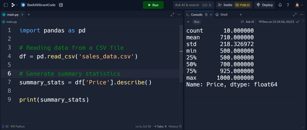
5. describe(): Calculate Summary Statistics for a Series or DataFrame

The describe() function generates descriptive statistics that summarize the central tendency, dispersion, and shape of a dataset’s distribution.

Example:

Let's generate summary statistics for the product prices.

# Generate summary statistics

summary_stats = df['Price'].describe()

print(summary_stats)

Explanation:

• df['Price'].describe(): Provides descriptive statistics for the Price column.

Output:

6. plot(): Plot a Series or DataFrame

The plot() function generates a plot of a Series or DataFrame. This is essential for visualizing data trends.

Example:

Let's plot the product prices over time.

import pandas as pd

import matplotlib.pyplot as plt

# Create a DataFrame with dates and prices

df = pd.DataFrame({

    'Date': ['2024-01-01', '2024-01-02', '2024-01-03', '2024-01-04', '2024-01-05'],

    'Price': [1000, 500, 700, 500, 1000]

})

# Convert 'Date' column to datetime

df['Date'] = pd.to_datetime(df['Date'])

# Plot the prices

df.plot(x='Date', y='Price', marker='o', title='Product Prices Over Time')

plt.xlabel('Date')

plt.ylabel('Price')

plt.show()

Explanation:

• pd.to_datetime(df['Date']): Converts the Date column to datetime format.

• df.plot(x='Date', y='Price', marker='o', title='Product Prices Over Time'): Plots the Price column against the Date column with markers and a title.

Output:

The plot will show the price of products over the specified dates with markers at each data point.

7. iloc: Selecting Rows and Columns by Index

The iloc function allows you to select rows and columns in a DataFrame by their index positions (integer-location based).

Example:

Let's select specific rows and columns from our DataFrame.

# Create a DataFrame

df = pd.DataFrame({

    'Product': ['Laptop', 'Tablet', 'Smartphone', 'Tablet', 'Laptop'],

    'Quantity': [1, 2, 3, 4, 5],

    'Price': [1000, 500, 700, 500, 1000]

})

# Select the first 3 rows and the first 2 columns

selected_data = df.iloc[0:3, 0:2]

print(selected_data)

Explanation:

• df.iloc[0:3, 0:2]: Selects the first 3 rows and the first 2 columns from the DataFrame.

Output:

Summary

These Pandas functions are essential tools for data analysis. They help you load, clean, analyze, and visualize data efficiently. By mastering these functions, you can enhance your ability to work with data and derive meaningful insights.

Ready for More Python Fun?

Subscribe to our newsletter now and get a free Python cheat sheet! Dive deeper into Python programming with more exciting projects and tutorials designed just for beginners.

Keep exploring, keep coding, and enjoy your journey into data analytics with Pandas!